
Vectors serve as building blocks in mathematics, science, and engineering.
Aiming to demystify their structure and function, the following content supports intuitive thinking while honoring mathematical precision.
Vectors offer tools to visualize motion, model change, and represent quantities with both magnitude and direction.
Applications stretch across physics, engineering, data science, and machine learning.
Problems involving multiple variables or dimensions often require vector-based approaches for both conceptual and computational clarity.
That is why we want to talk about how to tackle vectors in math in greater detail.
Visualizing Vectors
Grasping what vectors represent begins with how they are pictured. Visual intuition helps bridge abstract symbols with physical meaning.
Instead of focusing only on formulas, envisioning vectors as objects in space, complete with direction and length, lays the groundwork for more confident application.
Once the visual element is understood, computations and equations begin to feel more natural and grounded in reality.
Geometric Interpretation
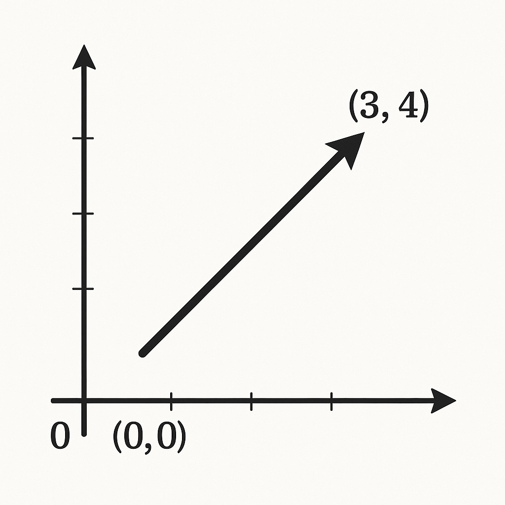
Imagine an arrow drawn on a flat surface, pointing from one location to another.
That arrow represents a vector. Its tail marks the starting point, and the arrowhead shows where it’s headed. Movement and direction are encoded into this one figure.
In two-dimensional space, vectors become easier to grasp. Picture a point moving from coordinates (0, 0) to (3, 4).
That change, captured by an arrow, has both direction and magnitude. Those features define what a vector is: a quantity that isn’t just a number but has orientation.
Vectors can represent displacement, velocity, force, or any quantity that involves both how much and in what direction.
On graphs or charts, their behavior is tracked as arrows with consistent length scaling and directionality. This perspective reinforces how vectors operate and interact in spatial environments.
Using i and j Unit Vectors
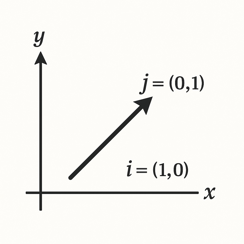
In 2D Cartesian coordinates, two unit vectors form the basis of all directional movement:
i = (1, 0)
j = (0, 1)
Any vector in the plane can be broken into these components. For example:
v = x·i + y·j
This means the vector shifts x units along the horizontal axis and y units along the vertical axis. Rather than thinking of vectors as single arrows, they are better understood as combinations of smaller, simpler movements in defined directions.
Component form allows vectors to be described clearly and manipulated easily.
Engineers, physicists, and data scientists use such breakdowns to simplify problems, solve equations, or simulate motion. You can find effective H2 Math tuition here, for example, for practical help on such vector breakdowns.
Vector Notation and Forms
Vectors can be written in different ways depending on context, discipline, or convenience. Being able to read and switch between these forms is essential for solving problems, interpreting data, or writing code.
Notation brings structure to how vectors are communicated and helps distinguish them from regular numbers or lists. Visual cues and formatting play a large role in ensuring clarity and accuracy.
Vector Representation

A vector can take several forms. One common version is the column vector, written vertically to emphasize its role in matrix operations or systems of equations:
[2
5
]
Another format is the component form, which places the values in parentheses to show direction and magnitude explicitly:
(2, 5)
Both of these forms represent the same vector—one that moves 2 units in the x-direction and 5 units in the y-direction.
Vectors can also be written using unit vectors. For example:
v = 2·i + 5·j
means two units along the x-axis and five along the y-axis.
Each format offers its own visual or structural benefit depending on the use case.
Standard Notations
Vectors are often distinguished using boldface, such as v, to signal that they are not scalars. In other cases, an arrow placed over the symbol, like →v, is used.
When typing in plain text or handwriting, alternatives such as underlines or tildes (~v) may be applied.
In textbooks or academic papers, consistent formatting helps reduce confusion. For people working with multiple vectors at once, clear and consistent notation avoids errors and saves time.
Notation in Programming vs Math
Caution is necessary when switching between math and programming. While math allows for the direct addition of two vectors:
(1, 2) + (3, 4) = (4, 6)
Some programming languages treat the expression differently. In Python, for example:
[1, 2] + [3, 4] will output [1, 2, 3, 4], not [4, 6].That’s because these brackets define a list, and the plus sign concatenates them. To perform correct vector arithmetic, specialized libraries like NumPy or MATLAB must be used.
These tools allow operations such as vector addition, scalar multiplication, and dot products to behave in line with mathematical expectations.
Misunderstanding notation in code can lead to major miscalculations. It’s important to ensure that the structures used match the math intended. Matching form and function reduces bugs and maintains consistency across fields like physics, engineering, and data science.
Basic Vector Operations
Vectors respond to operations in ways that mirror geometric movement.
Each operation, addition, subtraction, and scalar multiplication, has a clear visual and algebraic interpretation.
Mastering these lays the groundwork for understanding more complex ideas in physics, machine learning, and linear algebra.
Addition and Subtraction
Adding vectors involves placing one vector’s tail at the other’s head. The resulting vector starts at the original tail and ends at the final head. This process can be visualized as drawing two arrows in sequence.
The outcome creates the third side of a triangle or completes the diagonal of a parallelogram.
For example, consider:
- u = (2, 3)
- v = (1, 4)
- Then:
- u + v = (2 + 1, 3 + 4) = (3, 7)
Subtraction works by reversing the second vector and performing addition. Subtracting v from u means adding -v to u.
Geometrically, this flips v and connects its tail to the head of u, showing the difference between two positions.
u − v = (2, 3) − (1, 4) = (1, -1)
Both operations rely on the component-wise combination of x and y values, which makes them easy to compute and visualize.
Scalar Multiplication
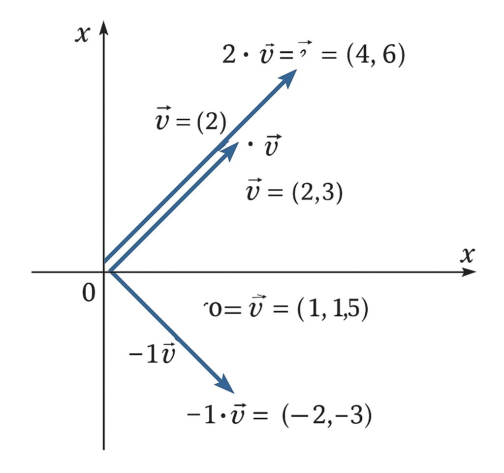
A scalar is a single number, and multiplying a vector by a scalar alters its size without changing its direction—unless the scalar is negative, in which case the vector flips.
Take vector v = (2, 3):
- 2·v = (4, 6) stretches it by a factor of 2
- 0.5·v = (1, 1.5) compresses it to half its original length
- -1·v = (-2, -3) flips it to point in the opposite direction
Scaling is especially useful when applying forces, adjusting magnitudes in simulations, or normalizing values in data processing.
Magnitude, Norm, and Distance
Quantifying vectors involves more than just knowing direction. Measuring their length or distance between them adds depth to analysis in physics, computer graphics, and data clustering.
Vector Magnitude (Length)
Magnitude reflects how long a vector is in n-dimensional space.
The most common way to compute this is using the Euclidean norm:
∥x∥ = √(x₁² + x₂² + … + xₙ²)
For a 2D vector (3, 4):
∥x∥ = √(3² + 4²) = √(9 + 16) = √25 = 5
Magnitude acts like a ruler measuring how far the vector stretches from the origin. It plays a key role in physics for evaluating speed, displacement, or energy, and in data science when comparing feature vectors.
Distance Between Vectors
To measure how far apart two vectors are, subtract one from the other and find the magnitude of the result:
∥p − q∥
Suppose p = (5, 2) and q = (1, 4), then:
p − q = (4, -2)
∥p − q∥ = √(4² + (-2)²) = √(16 + 4) = √20 ≈ 4.47
This formula gives the straight-line distance in space between two positions. It is essential in clustering, similarity detection, and optimization algorithms.
Advanced Insights (Optional for Beginners)
Some concepts deepen how vectors relate to angles, independence, and transformations. These insights help unlock more complex operations in applied math and science.
Dot Product and Angle Between Vectors
Dot product is a way to compare how two vectors align. It combines magnitudes with directional information:
a · b = ∥a∥ ∥b∥ cos(θ)
Where θ is the angle between vectors. If θ = 0, the vectors point in the same direction, and the dot product is maximized. If θ = 90°, the vectors are perpendicular, and the dot product is zero.
Dot product is foundational in physics for computing work, and in data science for calculating cosine similarity, which measures how similar two vectors are.
Linear Dependence and Independence
Vectors are linearly dependent if one can be obtained by scaling another. If no such relationship exists, they are independent.
For example:
- (2, 4) and (1, 2) are dependent since (2, 4) = 2·(1, 2)
- (2, 4) and (3, 5) are independent because no scalar links them exactly
In higher-dimensional spaces, independence ensures that vectors provide new directions or dimensions, which is key in solving systems of equations or building models with multiple variables.
Transformation and Applications

Vectors can represent anything measurable with multiple values—positions, stocks, forces, or pixel colors. A transformation modifies these values in predictable ways.
Example: A spreadsheet tracks monthly sales for different products. Applying a percentage growth across all months updates each row proportionally. That’s vector transformation in action.
Similarly, a portfolio vector with values (1000, 2000, 1500) may grow with a 10% market shift to become (1100, 2200, 1650). Each component changes according to the rule, preserving direction but altering magnitude.
This kind of transformation is key in graphics, economics, physics simulations, and neural networks.
Summary
Vectors introduce direction, scale, and structure into mathematical thinking. Concepts like component breakdown, operations, and distance lay the foundation for higher topics.
Visual thinking paired with consistent notation enables practical problem-solving in physics, engineering, and data science. Continued practice and analogy-driven learning reinforce comprehension.
Next steps may include matrices, linear transformations, or multivariable calculus for a deeper grasp of related topics.